You Only Look Once

Introduction to the architecture

Before YOLO, models like R-CNN used a two-stage approach: first proposing potential regions where objects might be, and then classifying those regions. YOLO changed the game by doing it all at once using a single Convolutional Neural Network (CNN). The main concepts behind YOLO:

• First the input image is divided into smaller regions of size .

• If the center of an object lands inside a specific grid cell, it is responsible for detecting it.

• Each cell predicts bounding boxes and confidence scores for these bouding boxes.

For a given grid cell, the network outputs a tensor containing the bounding box attributes and class probabilities. If you are predicting classes and bounding boxes per cell, the output dimension for each cell is . The values in each bounding box are:

• : coordinates relative the the center of the bounding box.

• : width and height of each bounding box relative the the whole image.

• : the confidence score (the probability that an object exists multiplied by the Intersection over Union (IoU) between the predicted box and the ground truth).

Math

To understand the internal processes, we need to look at how the model decodes bounding boxes and how it calculates its loss during training.

Bounding Box Prediction

Starting with YOLOv2, the model predicts bounding box coordinates using anchor boxes (predefined shapes). The network outputs parameterized coordinates (), which are transformed into bounding box coordinates () using the following equations:

where:

• is the sigmoid function assuring normalization to the interval .

• are the top-left coordinates of the current grid cell.

• are the width and height of the predefined anchor box.

Original Loss Function

The YOLO training process optimizes a massive, multi-part loss function. It computes the Sum of Squared Errors (SSE) across localization, objectness, and classification.

where:

• is a binary mask that is 1 if the -th bounding box in the -th cell is responsible for detecting the object, and 0 otherwise.

• The square root of width/height is used so that small deviations in small boxes are penalized more heavily than the same deviations in large boxes.

Training

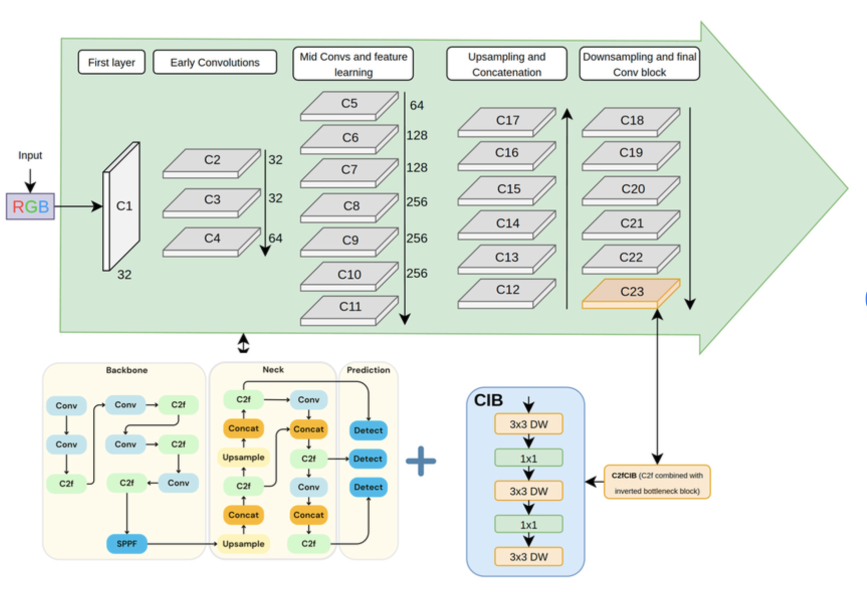
Forward Pass: The image is passed through the backbone (feature extractor) and the neck (feature aggregator), finally reaching the head where the grid predictions are made.

Target Assignment: The algorithm matches ground-truth objects to the specific grid cells and anchor boxes that have the highest IoU (Intersection over Union).

Loss Calculation: The model evaluates how far its predictions were from the ground truth using the loss functions (modern YOLOs use variations like CIoU loss for bounding boxes and Focal Loss for classification).

Backpropagation: The weights are updated using optimizers (like AdamW or, in YOLO26, MuSGD).

Post-Processing (Historically): Older YOLO models predicted thousands of boxes. They used Non-Maximum Suppression (NMS) to filter out overlapping boxes, keeping only the one with the highest confidence. Newer versions have engineered this step out entirely.

Evolution of SOTA

YOLOv1 (2015): The original paper by Joseph Redmon. Proved that single-stage detection was viable. It struggled with small objects and could only predict two boxes per grid cell.

YOLOv2 / YOLO9000 (2016): Introduced anchor boxes, high-resolution classifiers, and Batch Normalization. It could detect over 9000 classes.

YOLOv4 (2020): Alexey Bochkovskiy took over. Added Cross-Stage Partial Connections (CSPNet) and “Bag of Freebies” like Mosaic data augmentation, pushing speeds past 100 FPS on GPUs.

YOLOv5 (2020): Ultralytics natively ported YOLO to PyTorch. It introduced auto-learning bounding box anchors and hyperparameter evolution.

YOLOv6 & YOLOv7 (2022): Developed heavily for industrial and edge applications. YOLOv7 introduced the E-ELAN (Extended Efficient Layer Aggregation Network) architecture for better gradient flow.

YOLOv8 & YOLOv9 (2023–2024): YOLOv8 moved to an “anchor-free” architecture. YOLOv9 introduced Programmable Gradient Information (PGI) and the GELAN architecture to fix information bottlenecks in deep layers.

YOLOv10 & YOLO11 (2024): The era of NMS-free models began here. YOLOv10 introduced an end-to-end training strategy that eliminated the need for Non-Maximum Suppression, heavily reducing inference latency. YOLO11 optimized parameter efficiency for multi-tasking (segmentation, pose, tracking).

YOLO26 (Late 2025/2026): The current state-of-the-art by Ultralytics. YOLO26 is designed from the ground up for massive edge deployment and absolute simplicity:

• Native NMS-Free End-to-End Inference: It completely eliminates NMS natively in the architecture, making deployment on edge devices infinitely easier.

• MuSGD Optimizer: Inspired by breakthroughs in Large Language Models, it uses a hybrid of SGD and Muon for unparalleled training stability.

• DFL Removal: It removes Distribution Focal Loss to simplify hardware exports (like TensorRT and ONNX) without losing accuracy.

• ProgLoss + STAL: Advanced loss optimizations specifically engineered to make small-object detection highly accurate.

Dive into details

In this section we will explore some techonologies introduced by model authors to increase the performance of subsequent models.

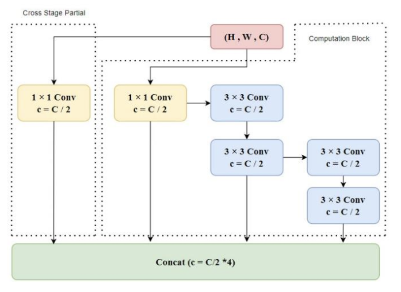
Cross-Stage Parial Networks (CSPNet)

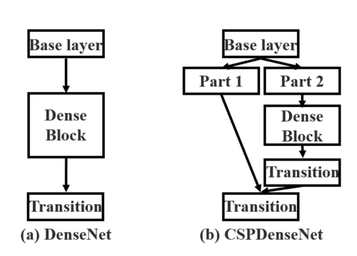
Before YOLOv4, architectures like ResNet and DenseNet were heavily used to extract features. Standard implementations suffer from duplicate gradient information. During backpropagation, the gradients of the exact same initial features are repeatedly computed and copied across mutltiple dense layers, which wastes the computation power. v4 integrated CSPNet into the Darknet backbone (creating CSPDarknet53) to solve this. In a standard DenseNet, the output of the -th layer is a function of all preceding feature maps concatenated together:

This means the weight updating equation for the -th layer heavily relies on over and over again. CSPNet modifies this by partitioning the base feature map into two parts along the channel dimension:

The first part, , completely bypasses the dense blocks. It is set aside to preserve the original gradient information. Only the second part, , goes through the computational bottleneck of the dense layers:

After dense layers, the output is passed through a transition layer to standardize the channels, producing . Finally, this is concatenated with the bypassed :

By splitting the channels in half, the number of parameters inside the dense block is reduced by roughly 50%. More importantly, because bypasses the block entirely, the gradient paths are strictly separated. The gradients for and are completely independent, which eliminates duplicate gradient flow and speeds up training while maintaining, or even boosting, accuracy.

Mosaic Data Augmentation

Standard data augmentation flips or crops a single image. Mosaic augmentation takes four different training images and stitches them together into a single grid. The description of boxes of course needs to be transoformed to fit into the new bounds of images.

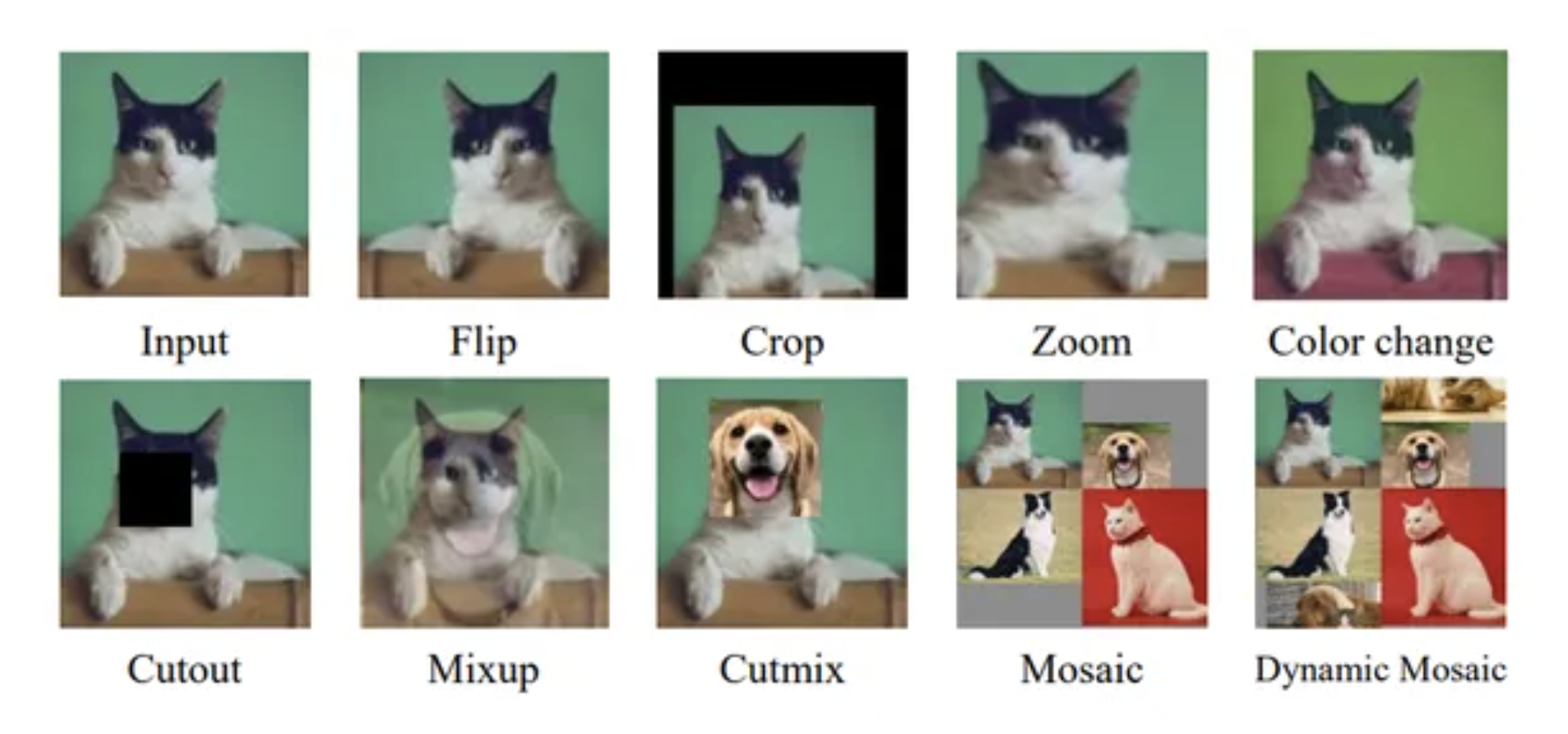
This forces the model to learn to identify objects at a much smaller scale (since the images are scaled down to fit the quadrant). Crucially, it allows Batch Normalization to calculate statistics across four entirely different image contexts simultaneously, significantly reducing the need for massive mini-batch sizes.

Complete Intersection over Union (CIoU Loss)

In earlier YOLO versions, the bounding box regression loss used Mean Squared Error (MSE) on the coordinates. This was flawed because a box of pixels and a box of pixels were penalized equally for a 5-pixel shift, even though the error is disastrous for the smaller box. YOLOv4 introduced Complete IoU (CIoU) loss to the Bag of Freebies, which considers three geometric factors: overlap area, central point distance, and aspect ratio.

The CIoU loss equation is defined as:

where:

• is the standard Intersection over Union between the predicted box and ground truth.

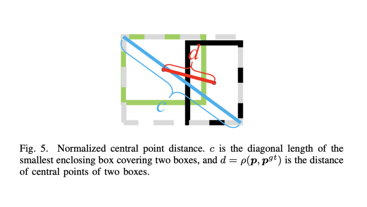
• is the Euclidean distance between the center points of the predicted box and ground truth box .

• is the diagonal length of the smallest enclosing box that covers both the predicted and ground truth boxes.

• is a mathematical measure of the consistency of the aspect ratio, calculated as:

• is a dynamic trade-off parameter that gives higher priority to the aspect ratio when the boxes are overlapping well:

This equation forces the network to not just overlap the boxes, but to perfectly align their centers and match their exact shape proportions.

GIoU - Generalized Intersection over Union

This loss function was also considered. It is based on the equation:

Here, and are the prediction and ground truth bounding boxes. is the smallest convex hull that encloses both and . is the smallest box covering and . The penality term in GIoU loss, will move the predicted box towards the target box in non-overlapping cases.

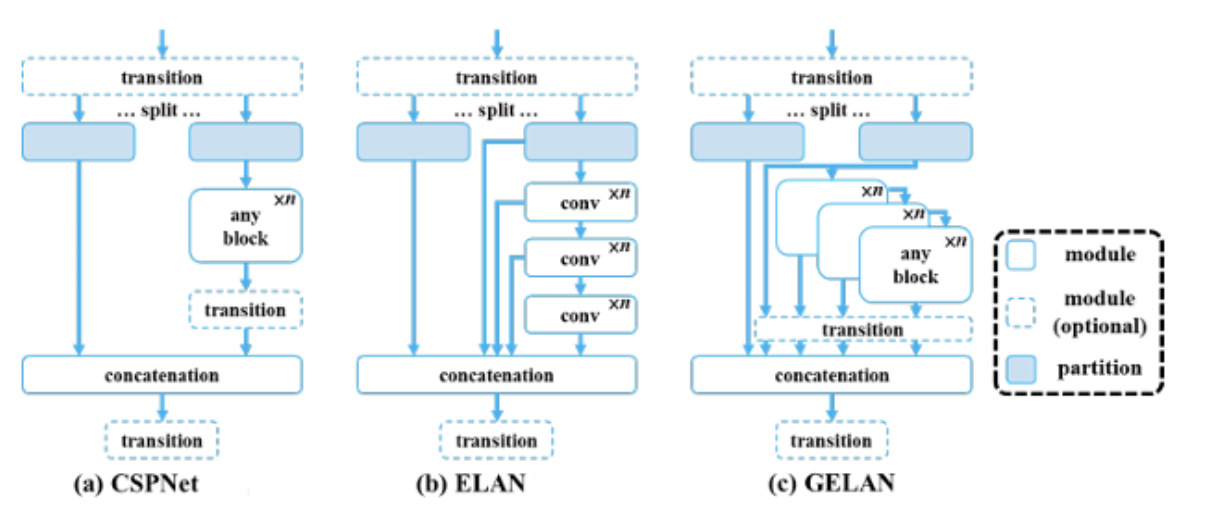
Extended Efficient Layer Aggregation Network (E-ELAN)

Before the “Extended” version, there was standard ELAN. ELAN was designed to solve the gradient degradation problem by optimizing how gradient paths are routed. Instead of just stacking layers endlessly (which creates a single, very long gradient path), ELAN creates multiple parallel branches of varying lengths. Some features pass through a short path (e.g., just one convolution), other features pass through a longer path (e.g., multiple stacked convolutions) and then at the end everything is concatenated. This guarantees that the network always has access to both a shortest gradient path (retaining original, undistorted information) and a longest gradient path (extracting highly complex features).

The problem with standard ELAN is that if you want to make the model smarter, you have to stack more computational blocks. Stacking more blocks eventually destroys the stable gradient paths that ELAN worked so hard to create. E-ELAN (Extended ELAN) solves this by changing how the network scales. Instead of making the network deeper (stacking more blocks), E-ELAN makes it “wider” by expanding the cardinality (the number of parallel groups or branches) without changing the underlying architecture of the computational blocks.

GELAN

Programmable Gradient Information (PGI)

Non-Maximum Suppression

DFL Removal

ProgLoss + STAL

Measuring YOLO Accuracy

In object detection, you cannot simply use standard “accuracy” (like you would in image classification) because predicting where an object is located is just as important as predicting what it is. To solve this, the industry standard relies on Average Precision (AP) and Mean Average Precision (mAP). Before calculating AP, we must define whether a bounding box prediction is correct. This is determined using IoU.

Based on an IoU threshold (), we categorize every prediction:

• True Positive (TP): A correct detection (IoU , correct class).

• False Positive (FP): An incorrect detection (IoU , or duplicate bounding box).

• False Negative (FN): A ground truth object that the model completely missed.

From those values we need to calculate two support metrics:

• Precision - out of all the objects the model claimed were positive, how many were actually positive.

• Recall - out of all the actual ground truth objects in the image, how many did the model found.

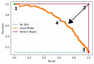
When a YOLO model predicts a bounding box, it also outputs a confidence score (e.g., 0.85 certainty that the box contains a car). If you set the confidence threshold very high (e.g., 0.90), the model only keeps predictions it is absolutely sure about. This results in high Precision (few False Positives) but low Recall (many False Negatives). If you lower the threshold to 0.10, the model predicts many boxes, resulting in high Recall but low Precision. Using by moving the threshold we can plot the Precision-Recall Curve.

Average Precision (AP) is the mathematical Area Under the Curve (AUC) of the Precision-Recall curve for a single specific class (e.g., only calculating AP for “dogs”). However, the raw PR curve is often jagged and noisy. To calculate the area reliably, we apply interpolation. Instead of using the exact Precision at a given Recall level, we use the maximum Precision found at that Recall level or any higher Recall level. The interpolated precision at a specific recall is defined as:

To calculate the final AP, we integrate the area under this smoothed curve using a Riemann sum across all recall points :

Where and are consecutive recall values when traversing the curve. While AP measures how well the model detects one specific class, Mean Average Precision (mAP) tells you how well the model performs across all classes. mAP is just the arithmetic mean of the AP values calculated for every class in the dataset.