We can describe a Machine Learning Model, as some highly convoluted mathematical function . Loss function measures how bad are the model’s predictions compared to expected labels given the input. Formally, given a target and a prediction under model parameters as , loss function would be describing similarity between them, as a number , where lower is better. In training we want to find optimal model parameters that minimize the empirical risk (average loss on data):
Backpropagation
Backpropagation is the chain rule applied to the computational graph to get gradients of a scalar loss with respect to all model parameters . Suppose that there is a node in graph that computes . Output is dependent both on input and layer parameters . Suppose that we know that the loss function has a gradient over the output of the layer described as , and we want to find both and . Then using the chain rule we can evaluate:
The matrix is sometimes referred to as Jacobian with entries .
Linear Layers
Linear Layer applies an affine map to each input vector:
The size of variables is as follows ( is the batch size): - , - , and - . Suppose that the layer received an upstream gradient equal to . Now we need to calculate partials w.t.r. to the layer’s weights and activation (). Using chain rule and tensor derivatives:
Doing the same for yields:
And for :
Activation Functions
Between the layers, we introduce activation functions to add non-linearity to the models. For each activation function we need to calculate both forward pass and derivative, so the flow of gradients through the model is undisturbed. Known activation functions are:
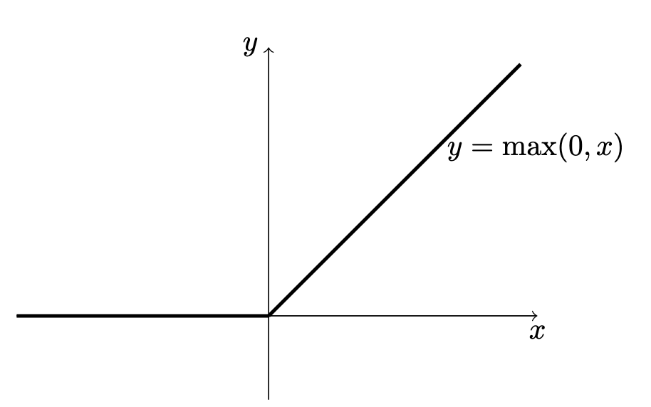
ReLU
For input and output can be defined as . Outflow of gradient will be the incoming gradient () into the layer times the derivative:
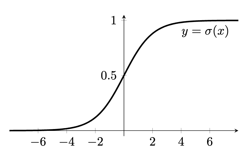
Sigmoid
This simple activation functions maps any real value to the valid probability range. Forward pass and backpropagation are defined as:
This is often used only for binary classification where value close to zero describes prediction of one class, and values close to one represent the other class.
Softmax
Softmax is a multidimensional sigmoid. Instead of normalizing one value to interval it normalizes vector of values so it represents a valid probability distribution. To satisfy this claim, each element needs to be greater that 0 and the sum of all elements must be equal to . Softmax is can also be denoted as . Calculating the gradients of give:
Building the Jacobian yields . Next we can build partial for entire vector :
This already is a nice form to implement because the element-wise sum of can be nicely casted along batches. Because , we can subtract current maximum value when calculating to increase numerical stability. Max operation needs to be done per object in the batch, not over the entire input matrix.
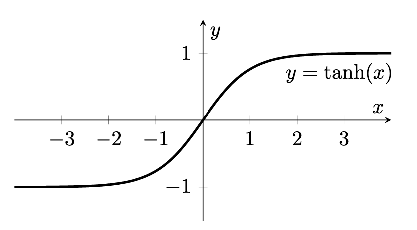
Hyperbolic Tangent
Inverse hyperbolic tangent activation can be described as , with outputs:
Plugging it in similar equation as in softmax function, gives:
The backpropagation step is reduced to simple element-wise operation on gradient and output of activation function.
Dropout
We can treat dropout as a standalone layer in the neural network. It applies a binary mask to the input tensor with a specified probability of \emph{keeping} single value equal to . The mask can be interpreted as a matrix . The output and the gradient of loss dependent on are:
We divide the output by to keep the expected activation equal. If we didn’t the network could fit to receiving lower values during training, and when the dropout is turned off (inferring the model) it would cause errors.
Optimizers
Optimizers help apply the gradients to the networks weights in order to find the global minimum. Technically we want to minimize the loss , so we tweak the model weights in the direction of negative gradient . In practice its impossible to make an update using entire training data, so we use batches. If we calculate cumulative gradient over a batch we arrive at SGD (Stochastic Gradient Descent).
Vanilla SGD
Given model parameters at time are , then the update is described as:
where represents the learning rate.
Momentum based
Momentum based optimizers introduce new parameter which represents \emph{stacked} velocity along gradients. This aggregation should makes the convergence faster, because the optimizer faster moves along areas with flat gradients.
where is the decay speed (or the aggregation) of the velocity.
Adaptive methods
Two known methods are AdaGrad and RMSProd. The latter introduces exponential moving averages of squared gradients which reduces oscillations.
Parameter is a linear interpolation of previous value and new square of gradients (power is taken element-wise). Then the gradients are normalized by dividing by the square root of geometric series of previous gradients. guards the division by .
Adam - mixed method
Method which merges both \textbf{Ada}ptive and \textbf{M}omentum approaches. The step is given by:
Here we introduce two LERP-ing terms which control the decay of momentum and square of gradients. Because we start with , the EMAs (Exponential Moving Averages) are biased toward during startup. This normalization negates this effect. If we apply weight decay to this equation, we arrive at AdamW optimizer algorithm.